What does the Brunt–Väisälä frequency tell you about a storm’s cap?
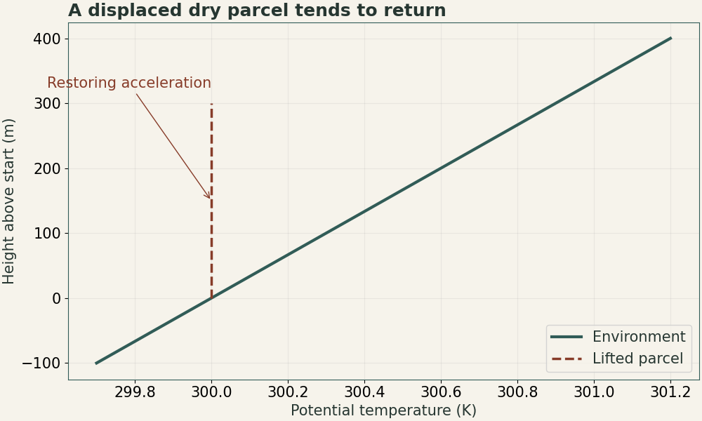
The dry Brunt–Väisälä frequency describes how rapidly a displaced air parcel oscillates in a stably stratified layer. Its square increases with the vertical potential temperature gradient under the dry assumptions.
Start with How do you calculate parcel buoyancy using virtual temperature?.
| Potential temperature gradient | N² (s⁻²) | Local dry response |
|---|---|---|
| +0.003 K/m | +9.81 × 10⁻⁵ | Restoring |
| 0 K/m | 0 | Neutral |
| −0.003 K/m | −9.81 × 10⁻⁵ | Displacement can grow |
Worked example
Displace a parcel upward by a small distance ξ with its potential temperature conserved. The environment changes by approximately ξ × dθ/dz. Buoyancy then acts as a restoring acceleration, approximately −(g/θ)(dθ/dz)ξ. Thus N² = (g/θ)dθ/dz. With g = 9.81 m/s², θ = 300 K and a gradient of 0.003 K/m, N² = 9.81 × 10⁻⁵ s⁻². N ≈ 0.00990 s⁻¹ and 2π/N ≈ 635 s. This local dry metric differs from signed CIN integrated over the parcel trajectory.
Practice questions
- Double the positive gradient and hold θ fixed. What happens to the period?
- If the gradient is negative, can you take √N² to get a real oscillation period?
Worked answers
Answer 1
N increases by √2. The period falls to 635/√2 ≈ 449 s.
Answer 2
The dry approximation gives negative N² and predicts growth of a small displacement. There is no real oscillation period for that case.
- N increases by √2. The period falls to 635/√2 ≈ 449 s.
- The dry approximation gives negative N² and predicts growth of a small displacement. There is no real oscillation period for that case.